While measurements with precision down to one μGal (one μGal is 10–8 ms–2) have been obtained at laboratory conditions for decades (e.g., Torge, 1989), recent advances have made it practically possible to carry out field surveys at such accuracy, and stationary measurement at sub-μGal precision. This increases the potential applications of gravity to smaller and deeper targets, with lower density contrasts and monitoring over shorter time-lapse intervals. High-precision measurements of gravity may be done by (A) absolute free-fall gravimeters, (B) quantum gravimeters (C) superconducting gravimeters, or (D) relative spring gravimeters. The various instruments all have their advantages and limitations. Some key properties are listed here.

Gravity instruments. A: Absolute FG5X, B: Absolute A-10, C: Quantum Gravimeter AQG, D: Super-conducting IGRAV, E: Spring-based CG-6, F: Spring-based ZLS.

Table: The most common gravity measurement techniques, and typical accuracies.
Absolute free-fall gravimeters measure the drop time of a mass in a vacuum chamber. These are immune to sensor drift. Repeated measurements are thus not required within a survey, and time-lapse changes can be seen without reference stations outside the area of interest. Semiportable instruments, the FG5 series, require setup and demobilization times of a few hours at an indoor site, and may give 2 μGal accuracy and 1 μGal repeatability. The smaller and more mobile A-10 instrument can give 10 μGal accuracy and repeatability in a 10 minutes reading on a quiet site. It can be operated outdoors at a wide range of temperatures (–18°C to +38°C).
Quantum gravimeters are based on atom interferometry (Menoret et al., 2018). The ACG has recently been designed for surveying, and it is still early to judge its performance compared to alternatives. Cooke et al. (2021) made the first evaluation for field surveys and found repeatability better than 5 µGal, sensitivity of 1-2 µGal after 1 hour of data collection and robustness to temperature changes at least up to +/- 5oC. This makes it of interest to test and evaluate further under field conditions.
Superconducting gravimeters measure a spherical superconducting mass, levitated using a magnetic force that exactly balances the force of gravity. The iGRAV requires a setup and sensor stabilization time of day(s), which makes it best suited for long continuous records on a site. Resolution is well below one μGal, and it is therefore particularly sensitive to measuring tides and atmospheric influence. Drift is less than 0.5 μGal/month, and scale factor will be stable within 10–2 for years (Calvo et al., 2014). Still, for monitoring over several years, drift uncertainty can build up to several μGal.
A relative spring gravimeter has a proof mass at the end of the spring, which extends proportional to the force of gravity and is accurately read off. CG-6 uses a quartz spring with a drift of some μGal/hour, while ZLS uses metal zero-length springs. Most of the drift is linear, and much of the residual drift can be controlled by repeated measurements during a survey. The scale factor needs to be calibrated from time to time. Repeatability is given at a few μGal. A seafloor version of the CG-3 and later CG-5 gravimeter was built for offshore monitoring (Sasagawa et al., 2003, Zumberge et al., 2008). A CG-6 update of the seafloor gravimeter is offered as ROVDOG III.5 or ROVDOG IV by Quad Geometrics.
Relative gravimeters can be used in campaigns/surveys, with one instrument doing sequential measurements at a grid of stations. Multiple visits and measurements at a site control drift and reduces some more random types of noise. The uncertainty in final station values can be significantly lower than the reading accuracy of each sensor, and repeatabilities of 1–2 μGal have been reported from several recent surveys (Vevatne et al., 2012; Eiken et al., 2017; Lien et al., 2017).
Gravity data need several corrections before station values and time-lapse changes can be estimated. Land data need to be corrected for variations in the groundwater (if not hydrology is the main target of the survey). Seafloor data need correction for the varying gravity attraction from the water above (sea level and seawater density, and in particular the ocean tides). All data need to be corrected for the varying gravity attraction from the atmosphere, earth tides, and ocean loading, either by a good model or by recordings at a reference gravimeter in the survey area.
Stability of measurement platforms over years is required for high-quality time-lapse data. This can be achieved by installing benchmarks, made of for instance massive concrete or a metal construction. In the North Sea, conical concrete benchmarks have been residing on the seafloor for more than 20 years (Stenvold et al., 2006). The gravity data can be corrected for height and height changes after the height has been measured, and an appropriate vertical gravity gradient has been applied.
A gravity monitoring program may be designed as a survey of an areal grid with relative or absolute gravimeter(s). A sparser grid of stations with permanent superconducting gravimeters may be an alternative, and surveys using a combination of gravimeters may be termed hybrid gravimetry.